Lesson 1 – The rules of axonometric projections
You can find this lesson’s content on this link.
- The rules of axonometric projections
When drawing objects, you must represent the 3-dimensional shape in a plane. This changes the dimensions and proportions of the object. In order for our drawing to be read by others, we have to follow certain rules. To represent the three-dimensional shapes in a plane, we will use projections. For engineers, technologists and skilled workers, knowledge of plane representation is essential. Until a part is made, it is only seen in its planar projections on a drawing board or screen.
1. Figure Oblique frontal dimetry
An axonometric image of a component is more similar to the image we see in space than to its image in a plane. By taking three axes, the dimensions of the object are plotted along the axes and the object is drawn. The scale along the axes can be constant, this is called one-dimensional axonometry. There are also ways of plotting where the dimensions along one axis are shortened (half the actual size is taken), these are called dimetric projections(two-dimensional axonometries) The angles enclosed by the axes also differ in each axonometric representation. The different axonometric representations are used to provide a more visual representation for easier recognition of the part.
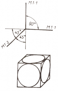
1.1. Oblique frontal dimetry
In this representation (Figure 1), the vertical and horizontal axes are perpendicular to each other and the extent of the object along these axes is scaled (M1:1). A size reduction is used along the oblique axis and the axis angel is usually 45° with the other two axes. If the interpretation is disturbed by the fact that a line of the part lies on the oblique axis, a 30° oblique axis may be used. This representation is also known as Kavalier axonometry. An oblique axonometric representation of a component is shown in Figure 2.
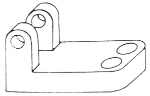
2. Figure Oblique dimetry of part
1.2. Rectangular Dimetry
In the dimetric or two-dimensional axonometry, the axes are oriented with a slope of 1:8 and 7:8 using auxiliary lines. These directions are taken by adding 8-8 units to the left and right of the horizontal auxiliary straight line from the origin. We then take 1 and 7 units downwards, respectively, to define a point on each axis, which we connect to the origin to obtain our oblique axes. The scale along the vertical and the 1:8 axis is a true scale (M1:1) and along the 7:8 axis a half scale (M1:2). As shown in Figure 3, the magnification of the drawing is 1.06, which gives a more true to scale sense. It is therefore preferred in engineering practice.
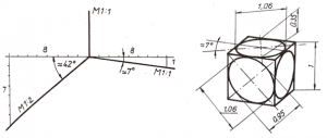
3. Figure Rectangular Dimetry
1.3. Rectangular Isometry
The picture planes axes are at 120° to each other and the scale is the same along the axes. The real lengths are measured along the axes. Figure 4 shows a cube in isometric view which have one unit long edges. It should be noted that the real dimensions of the object are only shown along the axes of the picture planes, the spatial elements are distorted. The image of the circles drawn on the faces of the cube in Figure 4, for example, becomes an ellipse in axonometry. The ellipse has a major axis of and a minor axis of 0.7. So the object is seen at 1.22 times magnification.
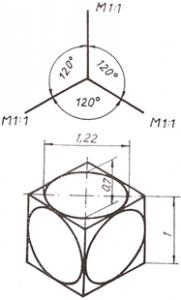
4. Figure Rectangular Isometry